mrpSteering

Executive Summary

The intend of this module is to implement an MRP attitude steering law where the control output is a vector of commanded body rates. To use this module it is required to use a separate rate tracking servo control module, such as rateServoFullNonlinear, as well.

Message Connection Descriptions

The following table lists all the module input and output messages. The module msg connection is set by the user from python. The msg type contains a link to the message structure definition, while the description provides information on what this message is used for.

Figure 1: mrpSteering() Module I/O Illustration

Module I/O Messages

Msg Variable Name	Msg Type	Description
guidInMsg	AttGuidMsgPayload	Attitude guidance input message.
rateCmdOutMsg	RateCmdMsgPayload	Rate command output message.

Detailed Module Description

The following text describes the mathematics behind the mrpSteering module. Further information can also be found in the journal paper Speed-Constrained Three-Axes Attitude Control Using Kinematic Steering.

Steering Law Goals

This technical note develops a new MRP based steering law that drives a body frame \({\cal B}:\{ \hat{\bf b}_1, \hat{\bf b}_2, \hat{\bf b}_3 \}\) towards a time varying reference frame \({\cal R}:\{ \hat{\bf r}_1, \hat{\bf r}_2, \hat{\bf r}_3 \}\). The inertial frame is given by \({\cal N}:\{ \hat{\bf n}_1, \hat{\bf n}_2, \hat{\bf n}_3 \}\). The RW coordinate frame is given by \(\mathcal{W}_{i}:\{ \hat{\bf g}_{s_{i}}, \hat{\bf g}_{t_{i}}, \hat{\bf g}_{g_{i}} \}\). Using MRPs, the overall control goal is

(1)\[ \pmb\sigma_{\mathcal{B}/\mathcal{R}} \rightarrow 0\]

The reference frame orientation \(\pmb \sigma_{\mathcal{R}/\mathcal{N}}\), angular velocity \(\pmb\omega_{\mathcal{R}/\mathcal{N}}\) and inertial angular acceleration \(\dot{\pmb \omega}_{\mathcal{R}/\mathcal{N}}\) are assumed to be known.

The rotational equations of motion of a rigid spacecraft with N Reaction Wheels (RWs) attached are given by Analytical Mechanics of Space Systems.

(2)\[[I_{RW}] \dot{\pmb \omega} = - [\tilde{\pmb \omega}] \left( [I_{RW}] \pmb\omega + [G_{s}] \pmb h_{s} \right) - [G_{s}] {\bf u}_{s} + {\bf L}\]

where the inertia tensor \([I_{RW}]\) is defined as

(3)\[[I_{RW}] = [I_{s}] + \sum_{i=1}^{N} \left (J_{t_{i}} \hat{\bf g}_{t_{i}} \hat{\bf g}_{t_{i}}^{T} + J_{g_{i}} \hat{\bf g}_{g_{i}} \hat{\bf g}_{g_{i}}^{T} \right)\]

The spacecraft inertial without the N RWs is \([I_{s}]\), while \(J_{s_{i}}\), \(J_{t_{i}}\) and \(J_{g_{i}}\) are the RW inertias about the body fixed RW axis \(\hat{\bf g}_{s_{i}}\) (RW spin axis), \(\hat{\bf g}_{t_{i}}\) and \(\hat{\bf g}_{g_{i}}\). The \(3\times N\) projection matrix \([G_{s}]\) is then defined as

(4)\[[G_{s}] = \begin{bmatrix} \cdots {}^{B}{\hat{\bf g}}_{s_{i}} \cdots \end{bmatrix}\]

The RW inertial angular momentum vector \({\bf h}_{s}\) is defined as

(5)\[h_{s_{i}} = J_{s_{i}} (\omega_{s_{i}} + \Omega_{i})\]

Here \(\Omega_{i}\) is the \(i^{\text{th}}\) RW spin relative to the spacecraft, and the body angular velocity is written in terms of body and RW frame components as

(6)\[\pmb\omega = \omega_{1} \hat{\bf b}_{1} + \omega_{2} \hat{\bf b}_{2} + \omega_{3} \hat{\bf b}_{3} = \omega_{s_{i}} \hat{\bf g}_{s_{i}} + \omega_{t_{i}} \hat{\bf g}_{t_{i}} + \omega_{g_{i}} \hat{\bf g}_{g_{i}}\]

MRP Steering Law

Steering Law Stability Requirement

As is commonly done in robotic applications where the steering laws are of the form \(\dot{\bf x} = {\bf u}\), this section derives a kinematic based attitude steering law. Let us consider the simple Lyapunov candidate function:

(7)\[ V ( \pmb\sigma_{\mathcal{B}/\mathcal{R}} ) = 2 \ln \left ( 1 + \pmb\sigma_{\mathcal{B}/\mathcal{R}} ^{T} \pmb\sigma_{\mathcal{B}/\mathcal{R}} \right)\]

in terms of the MRP attitude tracking error \(\pmb\sigma_{\mathcal{B}/\mathcal{R}}\). Using the MRP differential kinematic equations

(8)\[\begin{split} \dot{\pmb\sigma}_{\mathcal{B}/\mathcal{R}} &= \frac{1}{4}[B(\pmb\sigma_{\mathcal{B}/\mathcal{R}})] {}^{B}{\pmb\omega}_{\mathcal{B}/\mathcal{R}} \\ &= \frac{1}{4} \left[ (1-\sigma_{\mathcal{B}/\mathcal{R}}^{2})[I_{3\times 3} + 2 [\tilde{\pmb\sigma}_{\mathcal{B}/\mathcal{R}}] + 2 \pmb\sigma_{\mathcal{B}/\mathcal{R}} \pmb\sigma_{\mathcal{B}/\mathcal{R}}^{T} \right] {}^{B}{\pmb\omega}_{\mathcal{B}/\mathcal{R}}\end{split}\]

where \(\sigma_{\mathcal{B}/\mathcal{R}}^{2} = \pmb\sigma_{\mathcal{B}/\mathcal{R}}^{T} \pmb\sigma_{\mathcal{B}/\mathcal{R}}\), the time derivative of \(V\) is

(9)\[ \dot V =\pmb\sigma_{\mathcal{B}/\mathcal{R}}^{T} \left( {}^{B}{ \pmb\omega}_{\mathcal{B}/\mathcal{R}} \right)\]

To create a kinematic steering law, let \({\mathcal{B}}^{\ast}\) be the desired body orientation, and \(\pmb\omega_{{\mathcal{B}}^{\ast}/\mathcal{R}}\) be the desired angular velocity vector of this body orientation relative to the reference frame \(\mathcal{R}\). The steering law requires an algorithm for the desired body rates \(\pmb\omega_{{\mathcal{B}}^{\ast}/\mathcal{R}}\) relative to the reference frame make \(\dot V\) in Eq. (9) negative definite. For this purpose, let us select

(10)\[ {}^{B}{\pmb\omega}_{{\mathcal{B}}^{\ast}/\mathcal{R}} = - {\bf f}(\pmb\sigma_{\mathcal{B}/\mathcal{R}})\]

where \({\bf f}(\pmb\sigma)\) is an even function such that

(11)\[ \pmb\sigma ^{T} {\bf f}(\pmb\sigma) > 0\]

The Lyapunov rate simplifies to the negative definite expression:

(12)\[ \dot V = - \pmb\sigma_{\mathcal{B}/\mathcal{R}}^{T} {\bf f}(\pmb\sigma_{\mathcal{B}/\mathcal{R}}) < 0\]

Saturated MRP Steering Law

A very simple example would be to set

(13)\[ {\bf f} (\pmb\sigma_{\mathcal{B}/\mathcal{R}}) = K_{1} \pmb\sigma_{\mathcal{B}/\mathcal{R}}\]

where \(K_{1}>0\). This yields a kinematic control where the desired body rates are proportional to the MRP attitude error measure. If the rate should saturate, then \({\bf f}()\) could be defined as

(14)\[\begin{split} {\bf f}(\pmb\sigma_{\mathcal{B}/\mathcal{R}}) = \begin{cases} K_{1} \sigma_{i} &\text{if } |K_{1} \sigma_{i}| \le \omega_{\text{max}} \\ \omega_{\text{max}} \text{sgn}(\sigma_{i}) &\text{if } |K_{1} \sigma_{i}| > \omega_{\text{max}} \end{cases}\end{split}\]

where

\[\pmb\sigma_{\mathcal{B}/\mathcal{R}} = (\sigma_{1}, \sigma_{2}, \sigma_{3})^{T}\]

A smoothly saturating function is given by

(15)\[{\bf f}(\pmb\sigma_{\mathcal{B}/\mathcal{R}}) = \arctan \left( \pmb\sigma_{\mathcal{B}/\mathcal{R}} \frac{K_{1} \pi}{2 \omega_{\text{max}}} \right) \frac{2 \omega_{\text{max}}}{\pi}\]

where

(16)\[\begin{split} {\bf f}(\pmb\sigma_{\mathcal{B}/\mathcal{R}}) = \begin{pmatrix} f(\sigma_{1})\\ f(\sigma_{2})\\ f(\sigma_{3}) \end{pmatrix}\end{split}\]

Here as \(\sigma_{i} \rightarrow \infty\) then the function \(f\) smoothly converges to the maximum speed rate \(\pm \omega_{\text{max}}\). For small \(|\pmb\sigma_{\mathcal{B}/\mathcal{R}}|\), this function linearizes to

\[{\bf f}(\pmb\sigma_{\mathcal{B}/\mathcal{R}}) \approx K_{1} \pmb\sigma_{\mathcal{B}/\mathcal{R}} + \text{ H.O.T}\]

If the MRP shadow set parameters are used to avoid the MRP singularity at 360 deg, then \(|\pmb\sigma_{\mathcal{B}/\mathcal{R}}|\) is upper limited by 1. To control how rapidly the rate commands approach the \(\omega_{\text{max}}\) limit, Eq. (15) is modified to include a cubic term:

(17)\[ f( \sigma_{i}) = \arctan \left( (K_{1} \sigma_{i} +K_{3} \sigma_{i}^{3}) \frac{ \pi}{2 \omega_{\text{max}}} \right) \frac{2 \omega_{\text{max}}}{\pi}\]

The order of the polynomial must be odd to keep ${bf f}()$ an even function. A nice feature of Eq. (17) is that the control rate is saturated individually about each axis. If the smoothing component is removed to reduce this to a bang-band rate control, then this would yield a Lyapunov optimal control which minimizes \(\dot V\) subject to the allowable rate constraint \(\omega_{\text{max}}\).

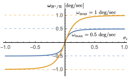
Figure 2: \(\omega_{\text{max}}\) dependency with \(K_{1} = 0.1\), \(K_{3} = 1\)

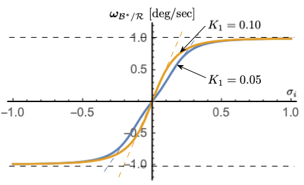
Figure 3: \(K_{1}\) dependency with \(\omega_{\text{max}}\) = 1 deg/s, \(K_{3} = 1\)

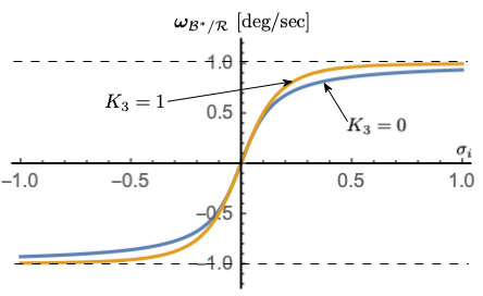
Figure 4: \(K_{3}\) dependency with \(\omega_{\text{max}}\) = 1 deg/s, \(K_{1} = 0.1\)

Figures 2-4 illustrate how the parameters \(\omega_{\text{max}}\), \(K_{1}\) and \(K_{3}\) impact the steering law behavior. The maximum steering law rate commands are easily set through the \(\omega_{\text{max}}\) parameters. The gain \(K_{1}\) controls the linear stiffness when the attitude errors have become small, while \(K_{3}\) controls how rapidly the steering law approaches the speed command limit.

The required velocity servo loop design is aided by knowing the body-frame derivative of \({}^{B}{\pmb\omega}_{{\mathcal{B}}^{\ast}/\mathcal{R}}\) to implement a feed-forward components. Using the \({\bf f}()\) function definition in Eq. (16), this requires the time derivatives of \(f(\sigma_{i})\).

\[\begin{split}\frac{{}^{B}{\text{d} ({}^{B}{\pmb\omega}_{{\mathcal{B}}^{\ast}/\mathcal{R}} ) }}{\text{d} t} = {\pmb\omega}_{{\mathcal{B}}^{\ast}/\mathcal{R}} ' = - \frac{\partial {\bf f}}{\partial \pmb\sigma_{{\mathcal{B}}^{\ast}/\mathcal{R}}} \dot{\pmb\sigma}_{{\mathcal{B}}^{\ast}/\mathcal{R}} = - \begin{pmatrix} \frac{\partial f}{\partial \sigma_{1}} \dot{ \sigma}_{1} \\ \frac{\partial f}{\partial \sigma_{2}} \dot{ \sigma}_{2} \\ \frac{\partial f}{\partial \sigma_{3}} \dot{ \sigma}_{3} \end{pmatrix}\end{split}\]

where

\[\begin{split}\dot{\pmb\sigma} _{{\mathcal{B}}^{\ast}/\mathcal{R}} = \begin{pmatrix} \dot\sigma_{1}\\ \dot\sigma_{2}\\ \dot\sigma_{3} \end{pmatrix} = \frac{1}{4}[B(\pmb\sigma_{{\mathcal{B}}^{\ast}/\mathcal{R}})] {}^{B}{\pmb\omega}_{{\mathcal{B}}^{\ast}/\mathcal{R}}\end{split}\]

Using the general \(f()\) definition in Eq. (17), its sensitivity with respect to \(\sigma_{i}\) is

\[\frac{ \partial f }{ \partial \sigma_{i} } = \frac{ (K_{1} + 3 K_{3} \sigma_{i}^{2}) }{ 1+(K_{1}\sigma_{i} + K_{3} \sigma_{i}^{3})^{2} \left(\frac{\pi}{2 \omega_{\text{max}}}\right)^{2} }\]

Module Assumptions and Limitations

This control assumes the spacecraft is rigid, and that a fast enough rate control sub-servo system is present.

User Guide

The following variables must be specified from Python:

• The gains K1, K3

• The value of omega_max

This module returns the values of \(\pmb\omega_{\mathcal{B}^{\ast}/\mathcal{R}}\) and \(\pmb\omega_{\mathcal{B}^{\ast}/\mathcal{R}}'\), which are used in the rate servo-level controller to compute required torques.

The control update period \(\Delta t\) is evaluated automatically.

Class MrpSteering

class MrpSteering : public SysModel

Data structure for the MRP feedback attitude control routine.

Public Functions

void reset(uint64_t callTime) override

This method performs a complete reset of the module. Local module variables that retain time varying states between function calls are reset to their default values.

Parameters:

callTime – The clock time at which the function was called (nanoseconds)

Returns:

void

void updateState(uint64_t callTime) override

This method takes the attitude and rate errors relative to the Reference frame, as well as the reference frame angular rates and acceleration

Parameters:

callTime – The clock time at which the function was called (nanoseconds)

Returns:

void

Public Members

double K1

[rad/sec] Proportional gain applied to MRP errors

double K3

[rad/sec] Cubic gain applied to MRP error in steering saturation function

double omega_max

[rad/sec] Maximum rate command of steering control

uint32_t ignoreOuterLoopFeedforward

[] Boolean flag indicating if outer feedforward term should be included

Message<RateCmdMsgPayload> rateCmdOutMsg

rate command output message

ReadFunctor<AttGuidMsgPayload> guidInMsg

attitude guidance input message

BSKLogger bskLogger = {}

BSK Logging.